Why People Stop Googling Marx in the Summer
Historic thinkers' legacy has a heartbeat—it's synchronized with the academic calendar.
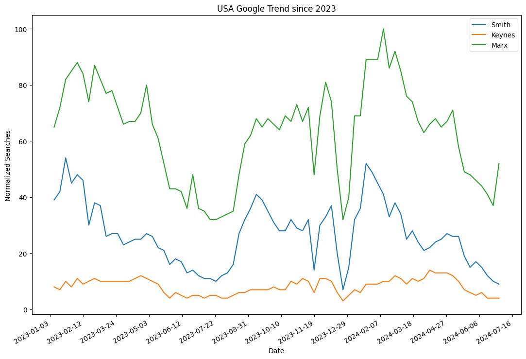
People search for Karl Marx more than Adam Smith or John Maynard Keynes. But all of these dead men have one thing in common: every year in the United States they are researched on a seasonal schedule that parallels the academic calendar. Google publishes search data by search terms and by “topic” on trends.google.com. The amount that people search any one of these men rises and falls with the others. They are closely correlated.
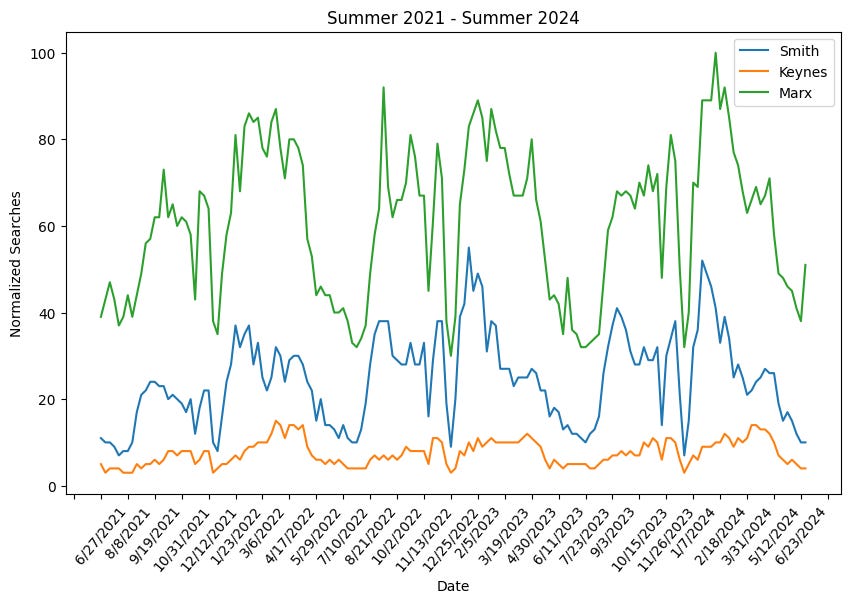
Here’s the data in the past year.
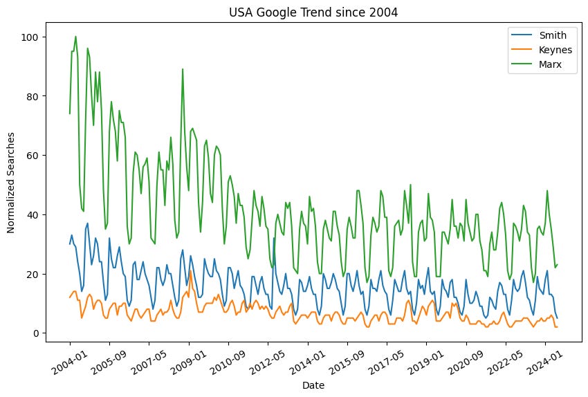
The cycle becomes even more apparent when zooming out.
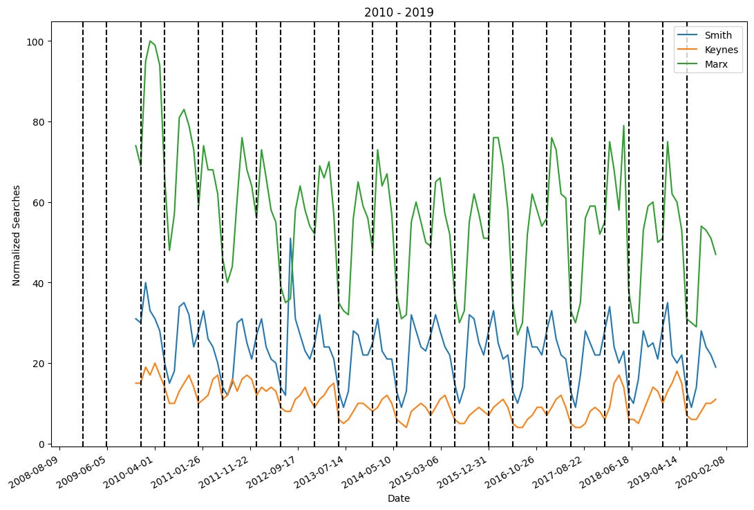
There are a few exceptions (apparently people were interested in Marx during 2020), but overall the search volume moves together. Drawing a vertical line each January 1st and June 1st confirms the seasonality. Looking at just the 2010s is where the cycle is clearest:
What third variable could be making these lines move together?
There are two consistent lows each year. One in summer and one in the winter. The summer decline is longer and more pronounced. The decline is the winter shorter, kind of like winter break. Notice the decline in the summer and winter months.
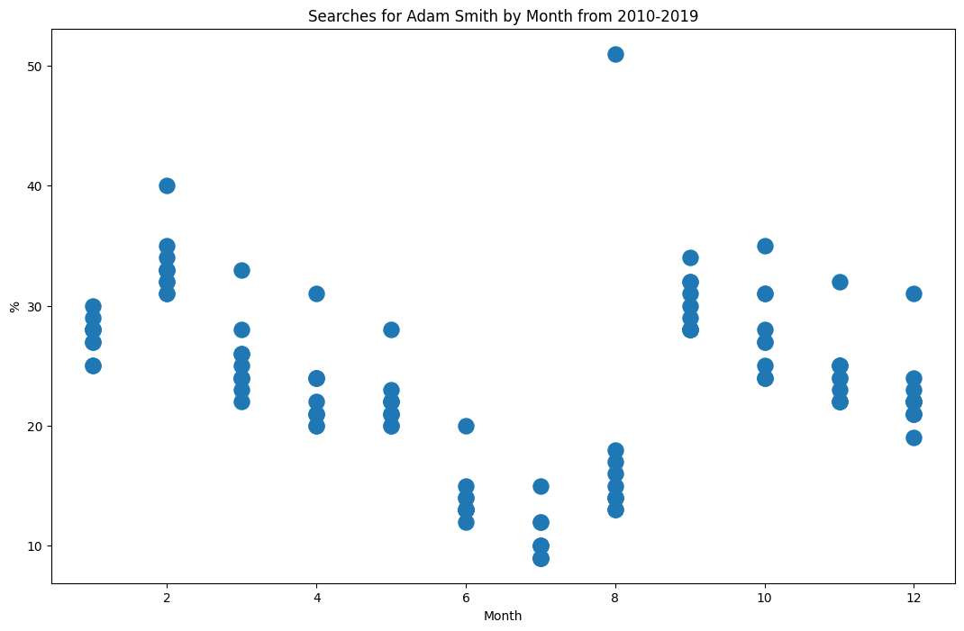
By Month
By graphing the trend for each month over the 2010 period shows a clear seasonality.
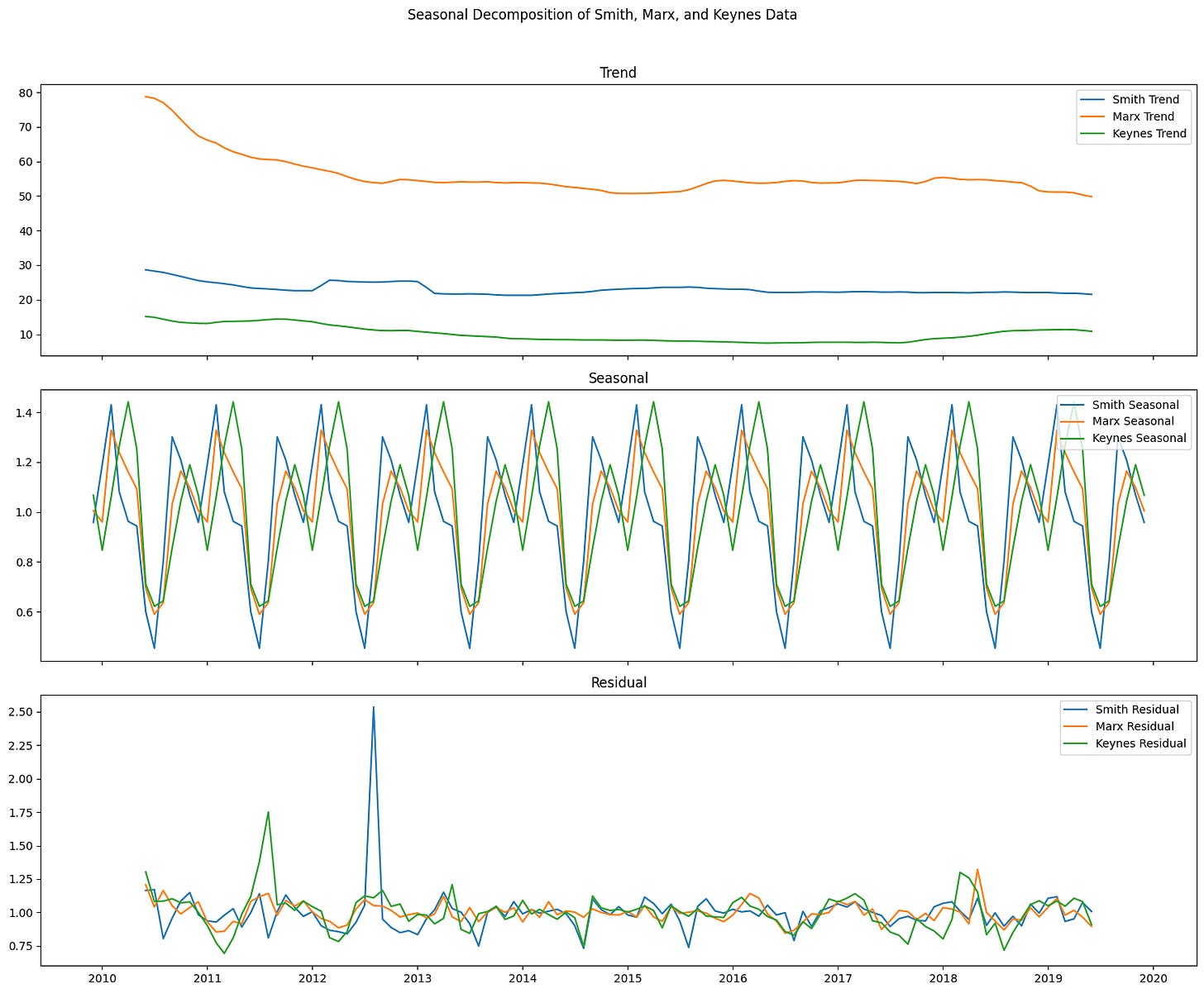
Time Series Seasonality and Trend
Yes, it is visible to the eye, but can we model it? As a disclaimer, I am new to time series analysis. This is by no means an exhaustive or entirely formal analysis. Consider this an attempt at Data Analysis not Data Science.
I am choosing to focus on December 2009 to December 2019. This time period is sufficiently broad, while avoiding COVID-19, the 2008 financial crisis, and the Search Engine Wars of the 2000s.
We can model the relationship with: Y[t] = T[t] *S[t] *e[t] where T is the trend, S is the seasonality, and e is an error term.
Model Testing
For this model to be worth anything, a few things should hold:
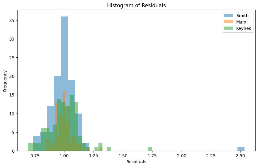
The residuals should have a normal distribution, meaning the distance from the actual values to the expected values in the model should be roughly normal.
No autocorrelation, which I take to mean the residuals of the search interest in one time period should not be largely determined by the search interest in the previous month. Admittedly, I’m unsure about the point of this one if I am trying to quantify seasonality in the first place, which is a type of autocorrelation.
Variance is homoscedastic, or constant for the entire time period. We cannot have the inaccuracy of predicted values varying greatly during different time periods.
A quick search gave me a few tests to run on to evaluate these three assumptions:
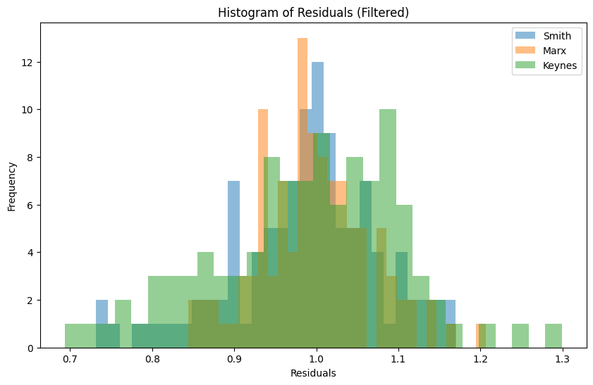
First off, the mean of the residuals is about 1 for each of the series, this is too be expected by construction, but we should test whether the distribution of the residuals is normal with the Shapiro-Wilk test. And the answer is definitely not! These p-values are LOW, less than an alpha of 0.05, so we reject the assumption that the residuals are normally distributed.
| | Smith | Keynes | Marx ||-----------|--------|--------|-------|| Statistic | 0.5215 | .9077 | .9584 || P-Value | 0.0000 | 0.0000 | .0018 |Visually, this makes sense. But what happens if we assume that any residuals above 1.3 are one off outliers, interesting in their own right, but probably outside shocks that we could drop.
| | Smith | Keynes | Marx ||-----------|--------|--------|-------|| Statistic | 0.5215 | .9077 | .9584 || P-Value | 0.0000 | 0.0000 | .0018 |Well now two of them could be assumed to be normal. That looks a little more believable. Maybe I’ll follow up to find out what caused those outliers.
The next test, the Ljung-Box, tests for autocorrelation within a series based on a number of lags. The question here is whether there is anymore “seasonality” remaining in the residuals? Here we started with 12 lags because our time period is that of the “month.” But the results hold on any lag from 2 to 12. The Smith residuals do not exhibit autocorrelation, while the Marx and Keynes models do.
| | Smith | Keynes | Marx ||-----------|---------|---------|---------|| Statistic | 14.4823 | 93.6141 | 44.2806 || P-Value | 0.2710 | 0.0000 | 0.0000 |Our final test, the Breusch-Pagan, tests for heteroscedasticity, meaning it is testing if the dispersion of the residuals remain constant. Each model passed this test, but Keynes was close.
| | Smith | Keynes | Marx ||-----------------|-------|--------|------|| LM Stat | 0.41 | 2.83 | 1.82 || LM Test p-value | 0.52 | 0.09 | 0.18 |
Overall, the testing shows a reasonable seasonality. Not perfectly in sync, but enough to accept the theory that the seasonality is due to the academic calendar.
The Significance of Seasonality
To some extent this is just a fun exercise, but I have two conclusions and a few lingering questions.
First, these thinkers are searched for at the same time in the United States every year. There is a clear seasonal pattern around the academic year. Second, they all follow that pattern. If one thinks that ideas matter, it is clear that the intellectual influence of past political economists fluctuates alongside the academic calendar. I think this shows that formal curriculum is vital to introducing individuals to the conversation of political economy.
Second, if every semester high-schools and universities across the US prompt people to try to learn something about Marx, Smith, or Keynes, the battle for ideas in the long run, may depend a lot on the resources available to the new student of political economy when they search for study resources each fall and spring.
Finally, I would like to know what caused the outliers. Why was there interest in Marx in 2020? Why is Marx researched less than in 2009?
What questions do you have? How could I make this analysis better?

